More Examples

This page contains further examples of applications of Python scripts to Astronomy beyond those in the Quick tour of Python:

Reading a table and plotting with asciitable

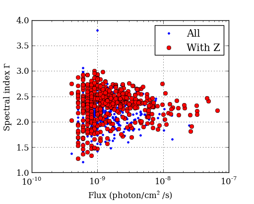
The Fermi Gamma-ray satellite has a nice catalog of AGN available through HEASARC. The script below will read in the catalog data using the asciitable module, do some basic filtering with NumPy, and make a couple of plots with matplotlib

import asciitable   # Make external package available

# Read table.
# ==> dat[column_name] and dat[row_number] both valid <==
dat = asciitable.read('fermi_agn.dat')

redshift = dat['redshift']    # array of values from 'redshift' column
flux = dat['photon_flux']
gamma = dat['spectral_index']

# Select rows that have a measured redshift
with_z = (redshift != -999)

figure(1)
semilogx(flux, gamma, '.b', label='All')  # First plot!
semilogx(flux[with_z], gamma[with_z], 'or', label='With Z')
legend(numpoints=1)
grid()
xlabel('Flux (photon/cm$^2$/s)')   # latex works
ylabel('Spectral index $\Gamma$')

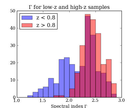
# Select low- and high-z samples
lowz = with_z & (redshift < 0.8)
highz = with_z & (redshift >= 0.8)

figure(2)
bins = arange(1.2, 3.0, 0.1)    # values from 1.2 to 3.0 by 0.1
hist(gamma[lowz], bins, color='b', alpha=0.5, label='z < 0.8')
hist(gamma[highz], bins, color='r', alpha=0.5, label='z > 0.8')
xlabel('Spectral index $\Gamma$')
title('$\Gamma$ for low-z and high-z samples')
legend(loc='upper left')

asciitable.write(dat[with_z], 'fermi_agn_with_z.dat')

Curve fitting with SciPy

SciPy provides curve_fit, a simple and useful implementation of the Levenburg-Marquardt non-linear minimization algorithm. This example shows a code to generate a fake dataset and then fit with a gaussian, returning the covariance matrix for parameter uncertainties.

from scipy.optimize import curve_fit

# Create a function
# ==> First encounter with *whitespace* in Python <==
def gaussian(x, a, b, c):
    val = a * exp(-(x - b)**2 / c**2)
    return val

# Generate fake data.
# Note: functions in random package, array arithmetic (exp)
n = 100
x = random.uniform(-10., 10., n)
y = exp(-(x - 3.)**2 / 4) * 10. + random.normal(0., 2., n)
e = random.uniform(0.1, 1., n)

# Fit
popt, pcov = curve_fit(gaussian, x, y, sigma=e)

# Print results
print "Scale =  %.3f +/- %.3f" % (popt[0], sqrt(pcov[0, 0]))
print "Offset = %.3f +/- %.3f" % (popt[1], sqrt(pcov[1, 1]))
print "Sigma =  %.3f +/- %.3f" % (popt[2], sqrt(pcov[2, 2]))

# Plot data
errorbar(x, y, yerr=e, linewidth=1, color='black', fmt=None)

# Plot model
xm = linspace(-10., 10., 100)  # 100 evenly spaced points
plot(xm, gaussian(xm, popt[0], popt[1], popt[2]))

# Save figure
savefig('fit.png')

The plotted fit result is as shown below:

Intermission: NumPy, Matplotlib, and SciPy

These three packages are the workhorses of scientific Python.

• NumPy is the fundamental package for scientific computing in Python [NumPy Reference]
• Matplotlib is one of many plotting packages. Started as a Matlab clone.
• SciPy is a collection of mathematical algorithms and convenience functions [SciPy Reference]

Synthetic images

This example demonstrates how to create a synthetic image of a cluster, including convolution with a Gaussian filter and the addition of noise.

import pyfits
from scipy.ndimage import gaussian_filter

# Create empty image
nx, ny = 512, 512
image = zeros((ny, nx))

# Set number of stars
n = 10000

# Generate random positions
r = random.random(n) * nx
theta = random.uniform(0., 2. * pi, n)

# Generate random fluxes
f = random.random(n) ** 2

# Compute position
x = nx / 2 + r * cos(theta)
y = ny / 2 + r * sin(theta)

# Add stars to image
# ==> First for loop and if statement <==
for i in range(n):
    if x[i] >= 0 and x[i] < nx and y[i] >= 0 and y[i] < ny:
        image[y[i], x[i]] += f[i]

# Convolve with a gaussian
image = gaussian_filter(image, 1)

# Add noise
image += random.normal(3., 0.01, image.shape)

# Write out to FITS image
pyfits.writeto('cluster.fits', image, clobber=True)

The simulated cluster image is below:

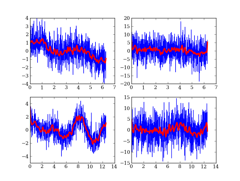
Running existing compiled codes

In addition to just doing computations and plotting, Python is great for gluing together other codes and doing system type tasks.

import os
import asciitable

smoothing = 30  # Smoothing window length
freqs = [2, 4]  # Frequency values for making data
noises = [1, 5] # Noise amplitude inputs

figure(1)
clf()

# Loop over freq and noise values, running standalone code to create noisy data
# and smooth it.  Get the data back into Python and plot.
plot_num = 1
for freq in freqs:
    for noise in noises:
        # Run the compiled code "make_data" to make data as a list of x, y, y_smooth
        cmd = 'make_data %s %s %s' % (freq, noise, smoothing)
        print 'Running', cmd
        out = os.popen(cmd).read()
        # out now contains the output from <cmd> as a single string

        # Write the output to a file
        filename = 'data_%s_%s' % (freq, noise)
        open(filename, 'w').write(out)

        # Parse the output string as a table
        dat = asciitable.read(out)

        # Make a plot
        subplot(2, 2, plot_num)
        plot(dat['x'], dat['y'])
        plot(dat['x'], dat['y_smooth'], linewidth=3, color='r')

        plot_num += 1

And much much more...

• Fast access to big (1e9 rows) tables with PyTables + HDF5
• 3-d plotting and surface rendering with Mayavi
• Sophisticated data modeling with advanced statistics with Sherpa
• Query VO tables and broadcast or retrieve tables to VO applications like TOPCAT.
• GUI application to quickly view thousands of X-ray survey image cutouts
• Python-based web site for browsing a complex multi-wavelength survey
• Thermal modeling of the Chandra X-ray satellite
• Interactive multi-user plots accessed through a web browser (!)
• Distributed computing with MPI for Python
• Make a little video distribution web site