Least-squares fitting in Python

Many fitting problems (by far not all) can be expressed as least-squares problems.

What is least squares?

• Minimise
• If and only if the data’s noise is Gaussian, minimising is identical to maximising the likelihood .
• If data’s noise model is unknown, then minimise
• For non-Gaussian data noise, least squares is just a recipe (usually) without any probabilistic interpretation (no uncertainty estimates).

scipy.optimize.curve_fit

curve_fit is part of scipy.optimize and a wrapper for scipy.optimize.leastsq that overcomes its poor usability. Like leastsq, curve_fit internally uses a Levenburg-Marquardt gradient method (greedy algorithm) to minimise the objective function.

Let us create some toy data:

import numpy

# Generate artificial data = straight line with a=0 and b=1
# plus some noise.
xdata = numpy.array([0.0,1.0,2.0,3.0,4.0,5.0])
ydata = numpy.array([0.1,0.9,2.2,2.8,3.9,5.1])
# Initial guess.
x0    = numpy.array([0.0, 0.0, 0.0])

Data errors can also easily be provided:

sigma = numpy.array([1.0,1.0,1.0,1.0,1.0,1.0])

The objective function is easily (but less general) defined as the model:

def func(x, a, b, c):
    return a + b*x + c*x*x

Usage is very simple:

import scipy.optimize as optimization

print optimization.curve_fit(func, xdata, ydata, x0, sigma)

This outputs the actual parameter estimate (a=0.1, b=0.88142857, c=0.02142857) and the 3x3 covariance matrix.

scipy.optimize.leastsq

Scipy provides a method called leastsq as part of its optimize package. However, there are tow problems:

• This method is not well documented (no easy examples).
• Error/covariance estimates on fit parameters not straight-forward to obtain.

Internally, leastsq uses Levenburg-Marquardt gradient method (greedy algorithm) to minimise the score function.

First step is to declare the objective function that should be minimised:

# The function whose square is to be minimised.
# params ... list of parameters tuned to minimise function.
# Further arguments:
# xdata ... design matrix for a linear model.
# ydata ... observed data.
def func(params, xdata, ydata):
    return (ydata - numpy.dot(xdata, params))

The toy data now needs to be provided in a more complex way:

# Provide data as design matrix: straight line with a=0 and b=1 plus some noise.
xdata = numpy.transpose(numpy.array([[1.0,1.0,1.0,1.0,1.0,1.0],
              [0.0,1.0,2.0,3.0,4.0,5.0]]))

Now, we can use the least-squares method:

print optimization.leastsq(func, x0, args=(xdata, ydata))

Note the args argument, which is necessary in order to pass the data to the function.

This only provides the parameter estimates (a=0.02857143, b=0.98857143).

Lack of robustness

Gradient methods such as Levenburg-Marquardt used by leastsq/curve_fit are greedy methods and simply run into the nearest local minimum.

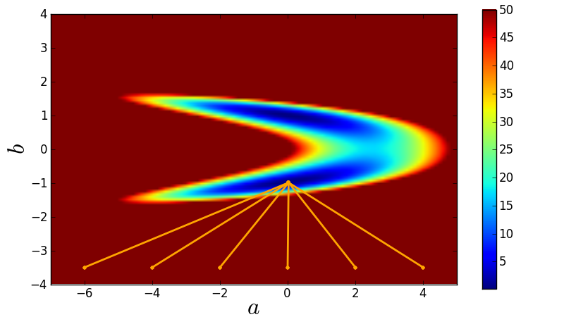
Here is the code used for this demonstration:

import numpy,math
import scipy.optimize as optimization
import matplotlib.pyplot as plt

# Chose a model that will create bimodality.
def func(x, a, b):
    return a + b*b*x  # Term b*b will create bimodality.

# Create toy data for curve_fit.
xdata = numpy.array([0.0,1.0,2.0,3.0,4.0,5.0])
ydata = numpy.array([0.1,0.9,2.2,2.8,3.9,5.1])
sigma = numpy.array([1.0,1.0,1.0,1.0,1.0,1.0])

# Compute chi-square manifold.
Steps = 101  # grid size
Chi2Manifold = numpy.zeros([Steps,Steps])  # allocate grid
amin = -7.0  # minimal value of a covered by grid
amax = +5.0  # maximal value of a covered by grid
bmin = -4.0  # minimal value of b covered by grid
bmax = +4.0  # maximal value of b covered by grid
for s1 in range(Steps):
    for s2 in range(Steps):
        # Current values of (a,b) at grid position (s1,s2).
        a = amin + (amax - amin)*float(s1)/(Steps-1)
        b = bmin + (bmax - bmin)*float(s2)/(Steps-1)
        # Evaluate chi-squared.
        chi2 = 0.0
        for n in range(len(xdata)):
            residual = (ydata[n] - func(xdata[n], a, b))/sigma[n]
            chi2 = chi2 + residual*residual
        Chi2Manifold[Steps-1-s2,s1] = chi2  # write result to grid.

# Plot grid.
plt.figure(1, figsize=(8,4.5))
plt.subplots_adjust(left=0.09, bottom=0.09, top=0.97, right=0.99)
# Plot chi-square manifold.
image = plt.imshow(Chi2Manifold, vmax=50.0,
              extent=[amin, amax, bmin, bmax])
# Plot where curve-fit is going to for a couple of initial guesses.
for a_initial in -6.0, -4.0, -2.0, 0.0, 2.0, 4.0:
    # Initial guess.
    x0   = numpy.array([a_initial, -3.5])
    xFit = optimization.curve_fit(func, xdata, ydata, x0, sigma)[0]
    plt.plot([x0[0], xFit[0]], [x0[1], xFit[1]], 'o-', ms=4,
                 markeredgewidth=0, lw=2, color='orange')
plt.colorbar(image)  # make colorbar
plt.xlim(amin, amax)
plt.ylim(bmin, bmax)
plt.xlabel(r'$a$', fontsize=24)
plt.ylabel(r'$b$', fontsize=24)
plt.savefig('demo-robustness-curve-fit.png')
plt.show()